This work was presented as the course final project for MIT 15.095: Machine Learning Under a Modern Optimization Lens, by Prof. Dimitris Bertsimas. A printer-friendly version of the whole report can be downloaded here, and a summary in the form of a poster can be found here. All the used code can be found at GitHub. Special thanks to my colleague and co-author of the project, Juan José Garau.

The project comprises the study of the application of predictive, optimization-based classification algorithms to a real-world task. Looking towards that aim, an online data science competition is the perfect medium due to both the availability of high-quality data, and the possibility of comparing different models and outcomes with the ones achieved by other participants using conventional heuristic methods. The online platform Kaggle is the most popular online competition organizer and 2019’s edition of the Data Science Bowl®(DSB) is a perfect fit for the objectives of this project.

Introduction

Online apps are a key element in the democratization of education all over the world, specially when it comes to early childhood education. Developing software focused to improve how kids learn is essential to make an impact on the users’ abilities and skills. In this year’s edition of the DSB, company PBS KIDS, a trusted name in early childhood education (3-5 years old) for decades, aims to gain insights into how media and game mobile apps can help children learn important skills for success in school and life. In this work, an optimization-based approach to understand the relationship between the educational content of the PBS KIDS Measure UP! app and how effectively its users learn is presented.

Problem statement

The app has a diverse range of educational material including videos, assessments, activities, and games. These are designed to help kids learn different measurement concepts such as weight, capacity, or length. The DSB challenge focuses on predicting players’ assessment performance based on the information the app gathers on each game session. Every detailed interaction a player has with the app is recorded in the form of an event, including things like mediacontent display, touchscreen coordinates, and assessment answers.

This data is highly fine-grained, as multiple events might be recorded in less than one second. With this data, the competition participants must predict the performance ofcertain assessments whose outcomes are unknown, given the history of a player up to that assessment. Based on the prediction, the goal is to classify the player into one of four performance groups, which represent how many attempts takes a kid to successfully complete the assessment. The aim of the challenge is to help PBS KIDS discover important relationships between engagement with high-quality educational media and learning processes, by understanding what influences the most on childrens’ performance and learning rate.

Figure 1. A look at PBS KIDS Measure Up! app.

We tackle the problem using a feature extraction process focused on exploiting the time series nature of the data and the application of different Optimal Classification Tree (Bertsimas & Dunn, 2019) models in order to both achieve a high predictive power and gain interpretable insights. Additionally, we provide two ideas of how this work could continue leveraging the potential of optimization-based machine learning methods.

Data Overview

The dataset provided by the competition is primarily composed of all the game analytics the PBS KIDS Measure UP! app gathers anonymously from its users. In this app, children navigate through a map and complete activities, video clips, games, or assessments (each of them considered a different game_session, and its nature expressed as type).

Each assessment is designed to test a child’s comprehension of a certain set of measurement-related skills. There are five assessments: Bird Measurer, Cart Balancer, Cauldron Filler, Chest Sorter, and Mushroom Sorter.

Data volume

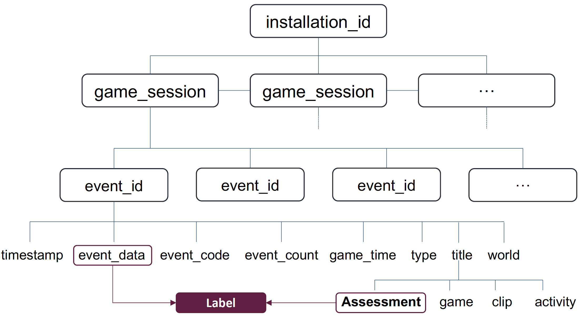
To help the reader understand the data, Figure 2 shows the tree-like structure of the dataset. Each application install is represented by an installation_id, which can be considered to map to one single user. The training set provides the full history of gameplay data of 17,000 installation_ids, while the test set has information for 1,000 players. Moreover, each installation_id has multiple game_sessions of different types (activities, games, assessments…). In total there are around 300,000 game_sessions in the training set and almost 30,000 in the test set.

Finally, each game_session is composed by several events that represent every possible interaction between the user and the app. These events are identified with a unique ID (event_id), and have associated data such as screen coordinates, timestamps, durations, etc, depending on the event’s nature. In total, there are around 11.3M events in the training set and 1.1M in the test set. We can conclude that the dimensionality of the problem is high and the data is presented in the form of dependencies and time series.

Figure 2. Dataset structure.

Classification labels

As previously introduced, the output of the model must be a prediction of the performance of the children in a particular assessment, in the form of a classification. The model should select one performance group out of four possible accuracy_groups. The groups are numbered from 0 to 3 and are defined as follows:

• accuracy_group3 : the assessment was solved on the first attempt
• accuracy_group2 : the assessment was solved on the second attempt
• accuracy_group1 : the assessment was solved after three or more attempts
• accuracy_group0 : the assessment was was never solved

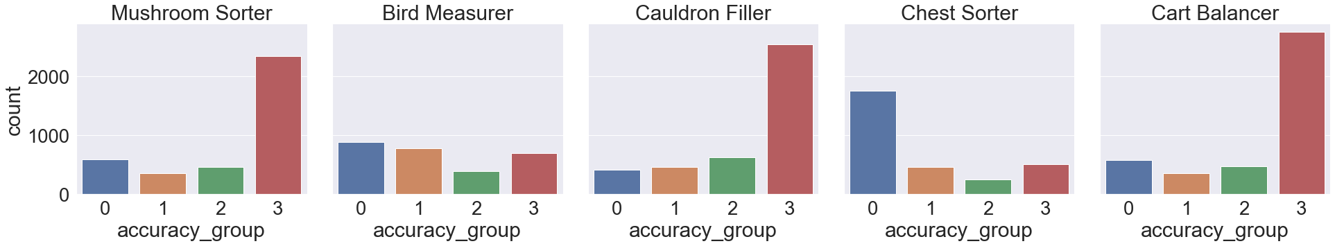
Figure 3 shows the distribution of the four possible accuracy_groups across the five assessments of the app. Notice that there are clearly three assessments that seem to be easier a priori as there is a majority of first-attempt correct answers, whereas one them has pretty much evenly distributed labels (Bird Measurer) and another one (Chest Sorter) seems to be more difficult than the others.

Figure 3. Prediction label distribution.

Training and test sets differences

Both training and test sets provided by the competition have similar structure in terms of the amount of information provided for each recorded event. The main difference is that all the information for each user (installation_id) in the test set stops at the beginning of an assessment, whose outcome is meant to be predicted.

However, in many cases, information from previous complete assessments is given. Every installation_id in the test has at least one assessment (the one to be labeled by the model), whereas many installation_id from the training set do not have any, and therefore have been removed from the dataset because they do not allow to generate any label for the training process. This leads to a major data volume decrease, as only 4242 installation_id out of the 17,000 original ones can be used.

Feature Engineering

The process of extracting features to train the machine learning model is time-consuming and challenging in this specific competition. Not only the provided data is in the form of a time series, but it also has a large amount of unnecessary information that needs to be filtered. In this section the process of transitioning from the original dataset to a dataset suitable to make predictions upon is explained.

Structuring data as time series

The test set comprises all historical data from different users prior to the first attempt of an assessment. Therefore, the time dimension is a key feature of this dataset, as only the events that have happened before each assessment can be considered for the definition of its associated features. This leads to the first step of the featuring engineering process: redefining the data for each player in order to leverage the time series structure of the original data.

Figure 4 shows how the original data is organized for a specific player (installation_id). Our approach is to transform all this information into multiple training data points that exploit the history of a player’s interactions with the app. Taking this approach allows training the model with only the information it is going to have available later in the prediction process, and avoids the fatal conceptual error of using future data for any assessment. It is also true that it leads to the deletion some of the available data, as any registered event happening after an assessment completion would not be used (see events to right of the second assessment in Figure 4).

Figure 4. (interactive) Time series representation of the game_sessions of a certain installation_id. The annotation above certain game_session shows the number of events they comprise (notice that all Clips (green) have only one event, as there is no recorded interaction with the player).

Training instance definition

When a player completes multiple assessments, multiple data points centered on each assessment can be considered. As observed in Figure 5, a training instance/data point is created from every assessment and its preceding information. The distribution of the number of assessments per user is very similar between the training and test sets, therefore, we can safely take all the events that happened prior to each assessment, and not only the ones between assessments. This allows to consider the whole experience of the user until the moment of facing that assessment, and therefore we can maximize the information input at every moment, without using future data.

Figure 5. Instance definition approach.

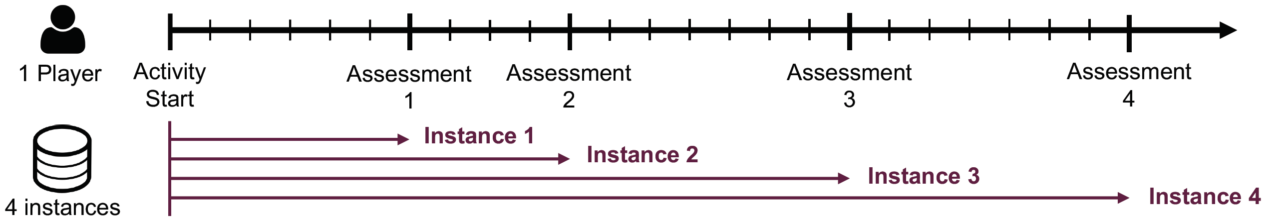
Overall, we can find approximately 21,000 assessments with this strategy, maximizing the number of training instances. In addition, this approach allows to generate extra training instances from the test set, as every completed assessment prior to the one whose outcome has to be predicted by the model can be considered as a new training instance with its associated label. This adds 2,549 more training instances to the final training dataset, summing up to a total of 23,788 rows.

Feature definition

The objectives of the feature creation approach are twofold: first, address how hard the particular assessment is by gathering assessment-related features from the whole data set. And second, determine how good a player is by looking at every recorded event before the start of an assessment and capturing skill-related features.

Assessment-related features

In order to provide the model with information regarding the difficulty of the assessment whose outcome has to be predicted, we compute both the mean and the median accuracy (continuous variable showing the percent of correct answers, different from the accuracy_group) as well as the mean and the median accuracy_group (discrete labels from 0 to 4 as it has been explained before). Even if they might be correlated, the optimization-based models that we use are not affected by this issue, and the metric that better describes the correlation between the difficulty of the assessment and the performance of the children will be automatically selected by the model.

As shown in Figure 3, some assessments are clearly easier than others. Therefore, we include both the assessment title and the world it belongs to (related to length, capacity or weight questions) as one-hot-encoded features. The latter is meant to provide some information on the type of questions the user is going to face, allowing the model to detect certain user profiles that are better at questions related with weight than at assessments covering capacity concepts, for example.

Player-related features

The largest proportion of the features associated to each assessment are the ones related to the historical data of the users. The purpose of all activities, videos, and games that each user is supposed (but not obliged) to do before taking the challenge of completing an assessment is to “train” a user to increase the chances of performing better at the assessment. Therefore, using information related to how the player performs at previous games or activities might be useful to make the prediction.

Seeking the quantification of how experienced each player is at the moment of each assessment, different metrics have been developed:

• Counters (every time a particular instance has been registered) of the different:
  • game_session by type (Assessment, Clip, Game, Activity)
  • game_session by title (all the possible games, activities, etc, the app includes)
  • event_code
  • game_session and event_code from the same world of the assessment to be predicted (gives a sense of the experience of the player with that particular family of concepts)
  • Times the player has already tried to complete the same assessment to be predicted, and its performance
• Total number of game_session and event_id
• Time played by game_session type, and total number of minutes played
• Average time spent per game_session type (gives a sense of how engaged and focused the player is)
• Average performance of the player in previous assessments
• Day of the week and time when the assessment has been completed

All the discrete features (e.g. accuracy group of the previously completed assessments) have been encoded as one-hot. After the feature engineering process, the final training dataset has 23,788 rows, 129 features and 4 possible classification outcomes. In the following section we explain which models are used to make predictions and how we can further leverage the data to better align ourselves with the purpose of the developer.

Optimal Classification Trees

Since the task is to predict the accuracy_group of a player before taking an assessment, in this work we focus on optimization-based classification models, namely Optimal Classification Trees (OCT). By means of Julia’s package Interpretable AI (IAI), in this section we train several OCT models and analyze their performance.

Models

Understanding the tradeoff between interpretability and predictive power they have, in this work we consider OCT models with both parallel and hyperplane (OCT-H) splits in order to gain insights on what makes users perform well and to obtain models capable of reaching high scores in the competition, respectively.

We understand the importance of training models with an appropriate selection of hyperparameters, therefore we carry out hyperparameter tuning tasks with a validation set before evaluating the performance of each model. In the case of OCT with parallel splits, we create a grid that considers three different values for the maximum depth parameter (5, 10, and 15) and three different values for the min bucket parameter (1, 5, and 10).

In the case of OCT-H, in order not to compromise runtime given the size of the dataset, we choose to fix the min bucket parameter to 1 and train two models with a maximum depth of 2 and 3, respectively. Since OCT-H considers hyperplane splits, and we decide not to enforce any sparsity constraint, choosing any other depth value beyond the selected ones does not provide impactful predictive power, degrades the interpretability of these models, and increases runtime unnecessarily.

All models are trained using the OptimalTreeClassifier with parallelization and using the misclassification error as the criterion to determine the best combination of hyperparameters. Additionally, we decide to duplicate the number of analyses and repeat both the OCT and OCT-H cases choosing to equally prioritize the 4 classes by means of the autobalance attribute. The rationale behind this decision can be easily understood by looking at Figures A1 and A2 in the Appendix. We cover the details of these figures in the coming section but the reader can notice that when autobalance is not used there is no leaf that predicts class 2. This is corrected when enforcing an equal importance among classes, helping understand the relationship between players’ behaviour and this class.

Predictive power

Tables 1 and 2 show the training and out-of-sample performance of the OCT and OCT-H models with and without the autobalance attribute. In this work we analyze the performance using two different metrics: on one hand we consider the accuracy, which takes into account the proportion of correctly classified labels; on the other hand we use the Cohen’s kappa coefficient with quadratic weights, which is the official metric of the competition and is defined as \[\kappa = 1 - \frac{\sum_{i=1}^k\sum_{j=1}^kw_{ij}x_{ij}}{\sum_{i=1}^k\sum_{j=1}^kw_{ij}m_{ij}}\] where \(x_{ij}\) represents the number of datapoints from class \(i\) that have been classified as class \(j\), \(m_{ij}\) is the expected number of datapoints from class \(i\) that have been classified as class \(j\), and finally \(w_{ij}\) is a weight factor defined as \[w_{ij} = 1 - \frac{i^2}{(j-i)^2}\]

By looking at the tables we can immediately appreciate the dominance of OCT-H models regardless of the use of the autobalance attribute. The autobalance feature works as expected, models without it perform better but that entails missing a class completely. This can be observed in figures A1 and A2 from the appendix, which do not have any leaf predicting class 2 (kids who solved the assessment in the second attempt).

Table 1. Training performance of OCT and OCT-H with and without the autobalance attribute.

Table 2. Out-of-sample performance of OCT and OCT-H with and without the autobalance attribute.

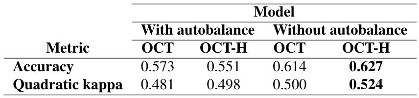
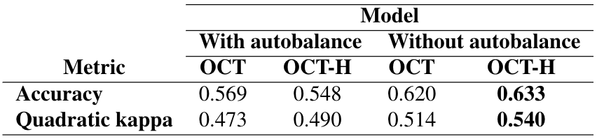
The model that achieves the best performance, both in terms of accuracy and the quadratic kappa coefficient, is OCT-H without balancing the outcome classes. Its kappa coefficient is 0.540, which at the moment this report is about to be submitted, is less than 0.03 points away from the first competitor in the leaderboard (with \(\kappa = 0.567\)). From a general perspective, only 90 competitors out of approximately 1900 (less than 5%) achieve better performance than our model. This result highlights the predictive potential of optimization-based classification trees.

Interpretability

While OCT-H allows us to obtain highly competitive models, OCT (with parallel splits) offers key insights to understand why kids perform differently when using the app. The resulting OCT decision trees, shown in Figures A1 and A2 from the appendix, highlight the relevance of specific groups of features:

• Which assessments: the presence of the variables is_Chest_Sorter, is_Cauldron_Filler, and is_Bird_Measurer shows us that the performance depends on which assessment is being done. The assessment Chest Sorter is identified as the hardest exercise and, when the player has not completed many assessments, Bird Measurer can also be challenging.
• Player’s experience: both decision trees include variables such as game_pct, ass_pct, and accumulated_accuracy_group. When this features reflect a player with more experience in games and assessments, the chances of predicting class 3 or 2 increase.
• Repeating an assessment: in the decision trees it is shown (features previous_completions and last_accuracy_same_title) that kids who are repeating an assessment are more likely to perform well.
• Specific events and titles: features 4020 and num_31 identify specific events and titles that, if present during an assessment, might alter the performance of the player.

In Figures A3 and A4 from the appendix we also show the decision trees obtained from the OCT-H models. In this case we have omitted the split decision due to the amount of variables included as a consequence of not having enforced sparsity.

Comparison to other models

Finally, we address the predictive performance of the OCT models compared to other popular approaches in data science competitions. Specifically, we train a XGBoost and a Logistic Regression model, both Python-based. Table 3 shows the accuracy and kappa coefficient performance, for both the training and test datasets, of these methods compared to the best OCT approach, namely the OCT-H model without the autobalance feature.

Table 3. Training and out-of-sample performance of OCT-H compared to Python’s _XGBoost_ and _Logistic Regression_.

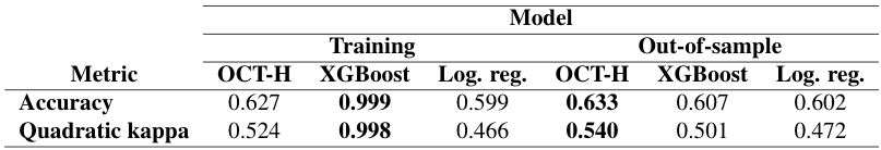
We can observe that OCT-H achieves a better performance than the other approaches, which helps to emphasize the relevance of optimization-based classification tree approaches. Using the same optimization procedure we have been able to both achieve competitive performance and understand the underlying relationship between how kids interact with the app and how successfully they learn the concepts.

Additional optimization-based approaches

Up to this point we have focused on the work that represents the goal of the DSB 2019: making predictions of players’ performance before taking on assessments. In this section we take a step further and focus on the goals that align the mission of the competition organizers: understand how to improve their products to enhance the learning experience for the kids.

To that end, following we broadly present two ideas based on optimization methods that could follow the work done in this project.

Optimal Splits

As presented in the previous section, in this work we have carried out hyperparameter tuning tasks by splitting the training dataset into actual train and validation data. While we have used randomization to split the data, we understand there might be better approaches considering the uniqueness of this data. As stated in the Data Overview section, there is a wide variety of games and activities kids can do before attempting to solve an assessment. Furthermore, since there is no obligation to take these intermediate steps, and there is no order enforced, the quantity of different player profiles and feature distributions is substantially high.

Consequently, when making random splits of the dataset, there is a high chance of obtaining unbalanced splits and not having an equal distribution of data points between the train and validation datasets. In order to solve this problem, we propose formulating a mathematical program to optimally split the dataset. This formulation, which is able to provide the optimal split regardless of the amount of splits to be created, is focused on reducing the discrepancies between the different groups. Since we are dealing with a dataset with more than one feature (129 to be precise), the formulation also takes into account multicovariates.

The function split_opt in the associated GitHub repository contains the code of this formulation in Julia. We propose a warm start based on the rerandomization split rule. Although we can’t provide results due to the dimensionality of the problem and runtime constraints, we understand this optimization-based procedure would allow us to obtain the best splits among data in order to increase the robustness of our models. In the end, making sure the models are robust is key to ensure the educational effectiveness of the app.

Optimal Prescription Trees

As part of possible extensions to this projects, it has also been considered the development of an Optimal Prescription Tree (Bertsimas & Dunn, 2019) model in order to provide a solution that would directly take actions based on the way the players use the app while they are using it. The model would achieve such task by taking into account both the performance prediction and the impact that every possible performance would cause.

Different possible prescription actions have been explored. The most promising one is the design of a certain learning path on the go. Since the app allows the user to freely decide its way through the game, one possible prescription could be whether to allow or to block the possibility of taking a particular assessment. The model would predict the performance that the player would have if he/she was allowed to do the assessment. If the historical data of the player led to a bad performance prediction, the prescription would be to take a particular activity or game that may help the user to gain more experience, and therefore blocking the possibility of trying to do the assessment at that moment.

The number of possible prescriptions for each different user and assessment scenarios have made unfeasible the task of looking for suitable prescription data given the time window of this project. However, with a larger dataset (approximately 1M assessments) and additional time, it could be possible to find cases to every possible prescription.

Conclusions and Future Work

In this work a new application of optimization-based machine learning methods has been explored. The highly-complex dataset provided by the competition organizers has allowed the creation of a large amount of features from a time series-oriented dataset. Then, based on this dataset two OCT and two OCT-H models have been very effective in terms of selecting the most important information and achieving a high score in the competition (top 5% at the moment this report is being written). This would have been much different if classical methods had been used instead. For instance, a long and arduous process of trial and error in terms of seeking the the different features that lead to a better prediction would have been needed.

We have proved the usefulness of optimization-based methods in prediction tasks and, more important, have provided insights on which factors affected the performance the most. We believe that in this particular problem the possibility of interpreting the prediction logic was key to align ourselves with the mission of the competition organizer.

Following this direction, we have opened the door to two additional optimization-based approaches that would additionally leverage the information obtained by the app to improve the learning experience of the players. Specifically, we have explored the idea of optimally splitting the dataset to ensure a higher degree of robustness and formulating a prescription problem in which the app takes into account the performance prediction to decide whether a user is ready or not to take certain assessments.

Appendix

Figure A1. (interactive) OCT without the autobalance setting.

Figure A2. (interactive) OCT with autobalance.

Figure A3. (interactive) OCT-H without the autobalance setting.

Figure A4. (interactive) OCT-H with autobalance.

References

Bertsimas, D., & Dunn, J. (2019). Machine learning under a modern optimization lens. Belmont, MA: Dynamic Ideas LLC. Available at: https://www.dynamic-ideas.com/books/machine-learning-under-a-modern-optimization-lens.